Excel: how to use the vlookup and hlookup functions

Excel has many features to create programs that are useful in everyday life. Whether for professional or personal needs, a simple spreadsheet can replace an entire application specially designed for a given task. In this tutorial, we will see how to use vlookup and hlookup functions in Excel.

Searchv et researchh are two of the most used functions in Excel. They are used to find data in a dense spreadsheet or even in external spreadsheets. Suppose you have an Excel sheet representing a company's customer database. Each customer has an identification (reference) and various data associated with their profile.

We want to create a formula to retrieve a customer's email after selecting their reference from an Excel drop-down list. One such possibility is through the use of the vsearch or hsearch function.

Vsearch and hsearch: how to use them?

Searchv and searchh in Excel allow, as their name suggests, to retrieve or search for information in a range of data and to return a value corresponding to this reference. A simply explained example is as follows: finds the customer whose reference is R03 in the beach A2 to D5 and get their email address. We will see how to translate this query into a formula in Excel.

But before getting to that, let's specify that the difference between vresearch and hresearch lies in the meaning of the search. V for vertical (column) and H for horizontal (row). Here's how to use them in a formula:

1. Lookupv(lookup_value; matrix; column; near_value)
2. Lookuph(lookup_value; matrix; row; near_value)

• Value sought : this is the value that must be sought in the range or matrix in order to fetch specific data concerning it
• Matrix : this is the range of cells in which the value to be searched is located
• Column or row number : this parameter corresponds to the number of the column (chevlookup) or row (hlookup) that contains the expected result. Count from the first column of the selected range, not the first column of the worksheet
• Close value : it is a logical (or boolean) argument that can only have two states: true or false. It is used to indicate whether you want to retrieve a result with a close value or an exact value corresponding to the sought_value. Very often, we are looking for a result corresponding exactly to the value sought. To do this, you must enter the False argument.

Also Read: How to Round Up or Down in Excel

Practical case

Finally, here is a concrete example that will help to better understand all these explanations. We are going to create a formula to fetch a customer's email address by entering their reference in a cell. To do this, we will use the vsearch formula since the references are listed one after the other vertically.

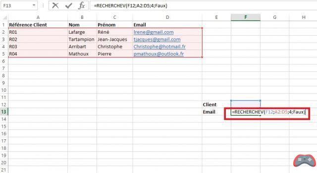
As you can see from the screenshot above, the formula looks like this: =VLOOKUP(F12;A2:D5;4;FALSE). We have the database (range of cells) on the one hand. It covers the first 5 rows of columns A to D.

Further down, in columns E and F, we created two rows to search for a value and return the corresponding result. In this case, cell F12 must contain the value to be searched for (customer reference). Cell F13 contains the formula to retrieve the customer's email.

• So the first argument of our formula is F12 since we will look for the reference entered in this cell
• The second argument is A2:D5 which corresponds to the range or matrix which contains both the reference and the value sought
• The third argument is the number 4 which corresponds to the index of the column that contains the sought result. In this case, the emails are in column D which is the 4th column starting from the first column of the selected range
• Finally, the FALSE argument is used to search for the exact match. It makes no difference here since it is a string.

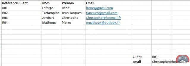
By validating the formula, the cell displays an N/A error, which is completely normal. To display a value, you must enter the reference of a customer in cell F12 to retrieve his email which will therefore be displayed in the cell containing the search formula (F13).

That's not very complicated. The operation is practically the same for the Findh function, which must be used if the list of the search source is arranged horizontally, which is not the case in our example.

The editorial advises you:

1. How to round in Excel (up or down)
2. How to password protect a Word or Excel document
3. Health pass: how to download it, where to use it, what you need to know

The ability to speed up or slow down a video on YouTube can be very useful. It was possible to do this in the web version of the platform for a while…Facebook allows you to deactivate the automatic playback of videos in your news feed. It's very simple, even if the path is not obvious to anyone who has never seen it...Google Chrome includes a reading mode that allows you to consult a page in optimal conditions. The functionality, however, is hidden in the bowels of the browser. In this tutorial,…It is easy to know if a contact has blocked you on WhatsApp, but some indicators can also trick you into believing it unfairly. So how do you know...